Convolutional neural networks for artistic style transfer

There’s an amazing app out right now called Prisma that transforms your photos into works of art using the styles of famous artwork and motifs. The app performs this style transfer with the help of a branch of machine learning called convolutional neural networks. In this article we’re going to take a journey through the world of convolutional neural networks from theory to practice, as we systematically reproduce Prisma’s core visual effect.

So what is Prisma and how might it work?

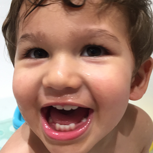
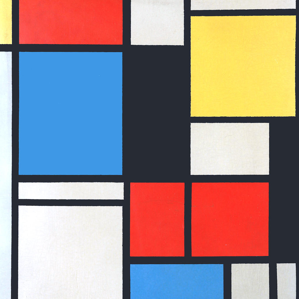
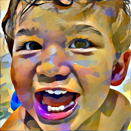
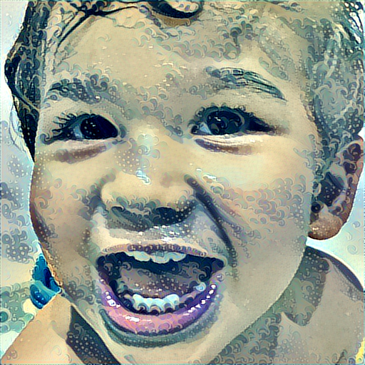
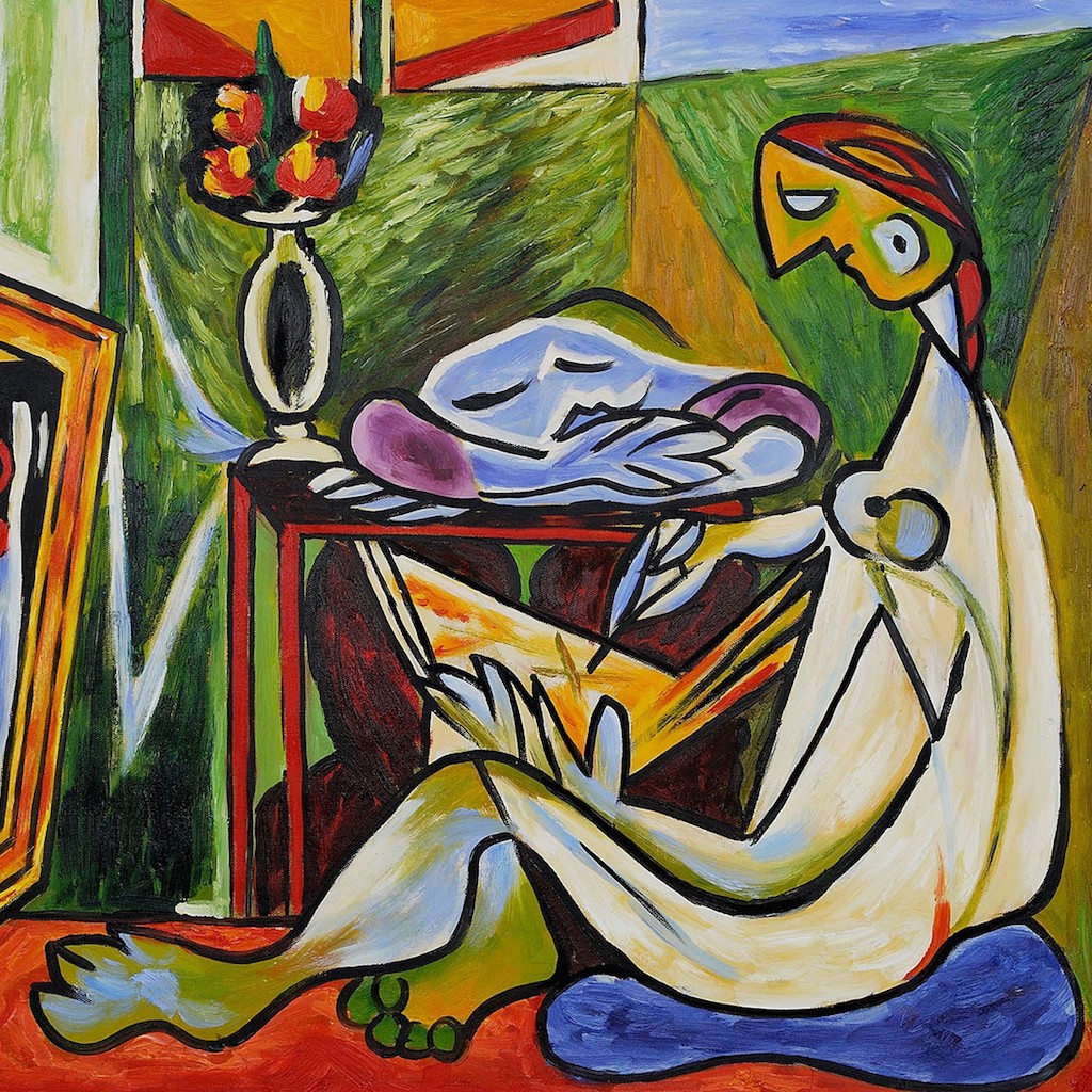
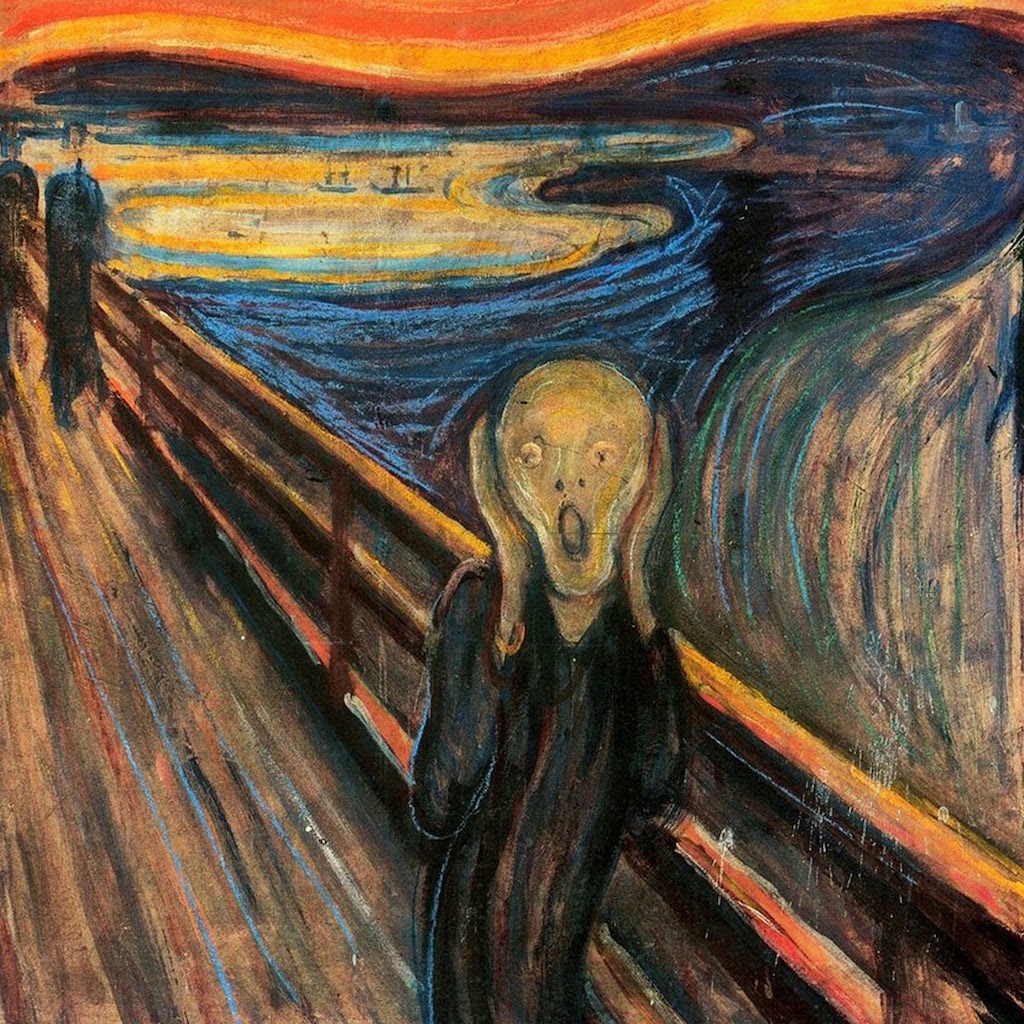
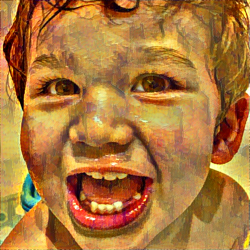
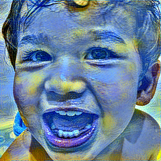
Prisma is a mobile app that allows you to transfer the style of one image, say a cubist painting, onto the content of another, say a photo of your toddler, to arrive at gorgeous results like these:

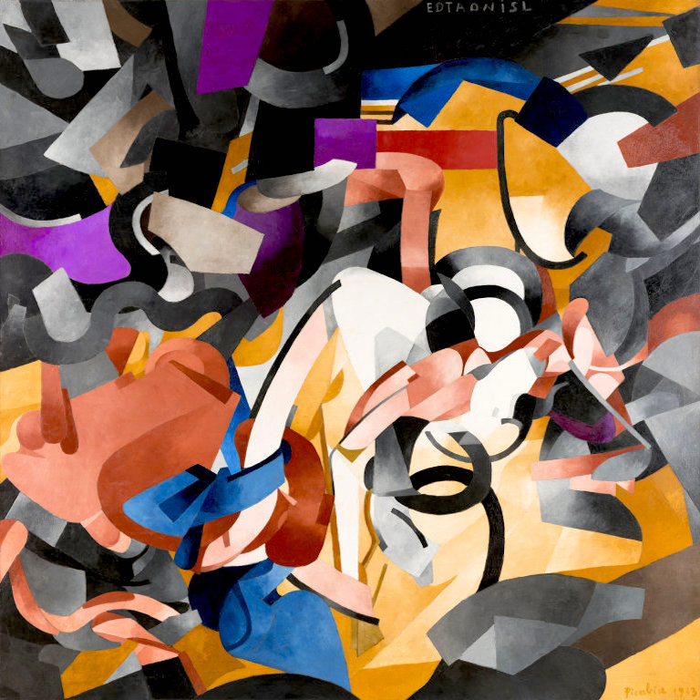
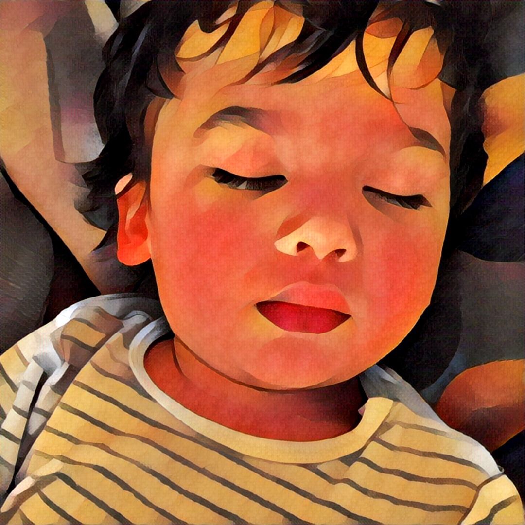
Like many people, I found much of the output of this app very pleasing, and I got curious as to how it achieves its visual effect. At the outset you can imagine that it’s somehow extracting low level features like the colour and texture from one image (that we’ll call the style image, $\mathbf{s}$) and applying it to more semantic, higher level features like a toddler’s face on another image (that we’ll call the content image, $\mathbf{c}$) to arrive at the style-transferred image, $\mathbf{x}$.

Now, how would we even begin to achieve something like this? We could perhaps do some pixel-level image analysis on the style image to get things like spatially-averaged colours or even aspects of its texture. But this brings up a deeper question: How do we go about explaining to our system that the texture and colour we’re interested in is at the scale of the brush strokes, not so much the overall shapes in the painting.

But let’s say we managed to do this anyway. How do we then selectively apply this style over the content? We can’t just copy and paste it without losing essential aspects of the content’s structure. Along the same lines, how do we cleanly discard the existing style of the content image?

I was stumped by many of these questions really early on, and as one does, turned to Google for help. My searches soon pointed me to a really popular paper (Gatys et al., 2015) that explains exactly how all this is achieved. In particular, the paper poses what we’re trying to do in mathematical terms as an optimisation problem.

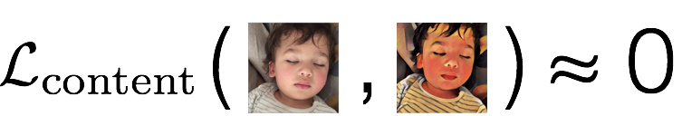
Let’s suppose that we had a way of measuring how different in content two images are from one another. Which means we have a function that tends to 0 when its two input images ($\mathbf{c}$ and $\mathbf{x}$) are very close to each other in terms of content, and grows as their content deviates. We call this function the content loss.

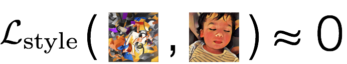
Let’s also suppose that had another function that told us how close in style two images are to one another. Again, this function grows as its two input images ($\mathbf{s}$ and $\mathbf{x}$) tend to deviate in style. We call this function the style loss.

Suppose we had these two functions, then the style transfer problem is easy to state, right? All we need to do is to find an image $\mathbf{x}$ that differs as little as possible in terms of content from the content image $\mathbf{c}$, while simultaneously differing as little as possible in terms of style from the style image $\mathbf{s}$. In other words, we’d like to simultaneously minimise both the style and content losses.

This is what is stated in slightly scary math notation below:

$$ \mathbf{x}^* = \underset{\mathbf{x}}{\operatorname{argmin}}\left(\alpha \mathcal{L}_{\mathrm{content}}(\mathbf{c}, \mathbf{x}) + \beta \mathcal{L}_{\mathrm{style}}(\mathbf{s}, \mathbf{x})\right) $$

Here, $\alpha$ and $\beta$ are simply numbers that allow us to control how much we want to emphasise the content relative to the style. We’ll see some effects of playing with these weighting factors later.

Now the crucial bit of insight in this paper by Gatys et al. is that the definitions of these content and style losses are based not on per-pixel differences between images, but instead in terms of higher level, more perceptual differences between them. Interesting, but then how does one go about writing a program that understands enough about the meaning of images to perceive such semantic differences?

Well, it turns out we don’t. At least not in the classic sense of a program with a fixed set of rules. We instead turn to machine learning, which is a great tool to solve general problems like these that seem intuitive to state, but where it’s hard to explicitly write down all the steps you need to follow to solve it. And over the course of this article, we’re going to learn just how to do this.

We start from a relatively classic place: the image classification problem. We’re going to slowly step through solutions of this problem until we’re familiar with a branch of machine learning that’s great for dealing with images called Convolutional Neural Networks (or convnets). We’re then going to see how convnets can be used to define these perceptual loss functions central to our style-transfer optimisation problem. We conclude with a concrete implementation of the solution of the problem (in Keras and TensorFlow) that you can play with and extend.

It is my hope that by starting our journey at a fairly basic place and gradually stepping up in complexity as we go along, that you get to learn something interesting no matter what your level of expertise.

Convolutional Neural Networks from the ground up

This section offers a brief summary of parts of the Stanford course Convolutional Neural Networks for Visual Recognition (CS231n) that are relevant to our style transfer problem. If you’re even vaguely interested in what you’re reading here, you should go take this course. It is outstanding.

The image classification problem

We begin our journey with a look at the image classification problem. This is a deceptively simple problem to state: Given an input image, have a computer automatically classify it into one of a fixed set of categories, say “baby”, “dog”, “car” or “toothbrush”. And the reason we’re starting with this problem is that it’s at the core of many seemingly unrelated tasks in computer vision, including our quest to reproduce Prisma’s visual effect.

In more precise terms, imagine a three channel colour image (RGB) that’s $W$ pixels wide and $H$ pixels tall. This image can be represented in a computer as an array of $D = W \times H \times 3$ numbers, each going between $0$ (minimum brightness) and $1$ (maximum brightness). Let’s further assume that we have $K$ categories of things that we’d like to classify the image as being one of. The task then is to come up with a function that takes as input one of these large arrays of numbers, and outputs the correct label from our set of categories, e.g. “baby”.

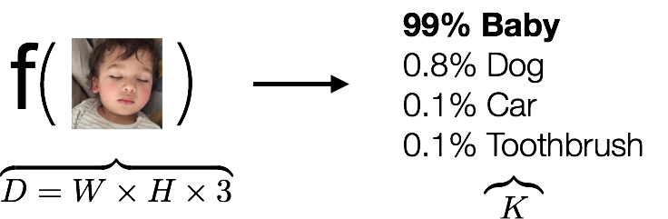
In fact, instead of just reporting one category name, it would be more helpful to get a confidence score for each category. This way, we’ll not only get the primary category we’re looking for (the largest score), but we’ll also have a sense of how confident we are with our classification. So in essence, what we’re looking for is a score function $\mathbf{f}: \mathbb{R}^D \mapsto \mathbb{R}^{K}$ that maps image data to class scores.

How might we write such a function? One naïve approach would be to hardcode some characteristics of babies (such as large heads, snotty noses, rounded cheeks, …) into our function. But even if you knew how to do this, what if you then wanted to look for cars? What about different kinds of cars? What about toothbrushes? What if our set of $K$ categories became arbitrarily large and nuanced?

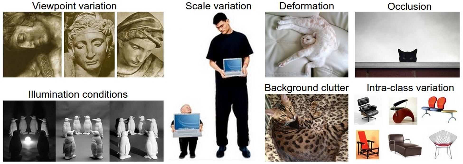
To further complicate the problem, note that any slight change in the situation under which the image was captured (illumination, viewpoint, background clutter, …) greatly affects the array of numbers being passed as input to our function. How do we write our classification function to ignore these sorts of superfluous differences while still giving it the ability to distinguish between a “baby” and a “toddler”?

These questions have the same flavour of difficulty as defining perceptual differences for the style transfer problem we saw earlier. And the reason for this is that there is a semantic gap between the input representation for images (an array of numbers) and what we’re looking for (a category classification). So we give up on trying to write this classification function ourselves, and instead turn to machine learning to automatically discover the appropriate representations needed to solve this problem for us.

This concept is the intellectual core of this article.

A supervised learning approach to the image classification problem

The branch of machine learning we turn to solve the image classification problem is called supervised learning. In fact, when you hear most people talking about machine learning today (deep learning or otherwise), what they’re probably referring to is supervised learning, as it is the subset of machine learning that has demonstrated the most success in recent years. Supervised learning is now the classic procedure for learning from data, and it is outlined below in the context of the image classification problem:

1. We start with a set of pre-classified example images, which means we have a set of images with known labels. This is called the training data, and these serve as the ground truth that our system is going learn from.

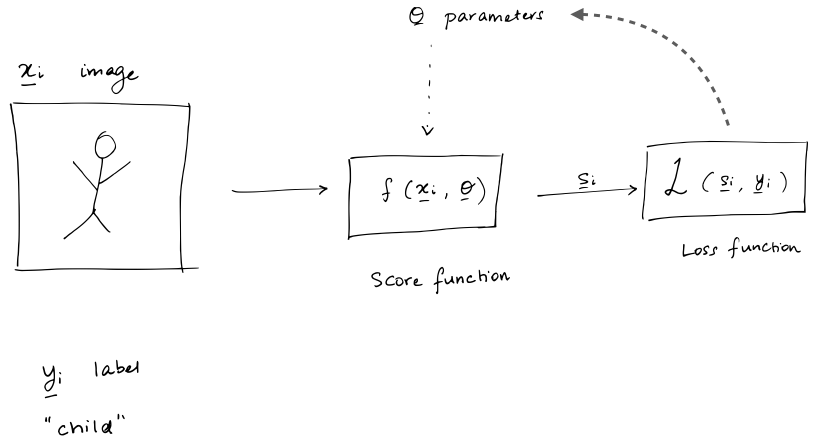
2. The function we’re trying to find is called the score function, which maps a given image to category scores. To define what we’re looking for, we first make a guess for its functional form and have it depend on a bunch of parameters $\mathbf{\theta}$ that we need to find.

3. We introduce a loss function, $\mathcal{L}$, which quantifies the disagreement between what our score function suggests for the category scores and what our training data provides as the known truth. Thus, this loss function goes up if the score function is doing a poor job and goes down if it’s doing great.

4. And finally, we have a learning or optimisation algorithm. This is a mechanism to feed our system a bunch of training data, and have it iteratively improve the score function by tweaking its parameters $\mathbf{\theta}$. The goal of the learning process is determine parameters that give us the best (i.e. lowest) loss.

Once we’ve completed this process and learnt a suitable score function, we hope that it generalises well. That is, the function works well for general input (called test data) that it hasn’t seen before.

Much of the excitement around machine learning today stems from making specific choices for these different pieces, allowing us to learn powerful functions that map a diverse set of inputs and outputs. And in what follows, we’re going to make increasingly sophisticated choices for these pieces aimed at incrementally better solutions to the image classification problem.

The linear image classifier

Recall the classification problem we’re trying to solve. We have an image $\mathbf{x}$ that’s represented as an array of numbers of length $D$ ($= W \times H \times d$, where $d$, the colour depth, is $1$ for a greyscale image and $3$ for an RGB colour image). We want to find out which category (in a set of $K$ categories) that it belongs to. So what we’re really looking for is a score function $\mathbf{f}: \mathbb{R}^D \mapsto \mathbb{R}^{K}$ that maps image data to class scores.

The simplest possible example of such a function is a linear map:

$$ \mathbf{f}(\mathbf{x}; \mathbf{W}, \mathbf{b}) = \mathbf{W}\mathbf{x} + \mathbf{b}, $$

which introduces two parameters we need to learn: a matrix $\mathbf{W}$ (of size $K \times D$, called the weights) and a vector $\mathbf{b}$ (of size $K \times 1$, called the biases).

Since we want to interpret the output vector of this linear map as the probability for each category, we pass this output through something called a softmax function $\sigma$ that squashes the scores to a set of numbers between 0 and 1 that add up to 1.

$$ s_j = \sigma(\mathbf{f})_j = \frac{e^{f_j}}{\sum_{k=1}^K e^{f_k}} $$

Let’s suppose our training data is a set of $N$ pre-classified examples $\mathbf{x_i} \in \mathbb{R}^D$, each with correct category $y_i \in 1, \ldots, K$. A good functional form to determine the total loss across all these examples is the cross entropy loss:

$$ \mathcal{L}(\mathbf{s}) = - \sum_i log(s_{y_i}) $$

For each example, this function simply plucks the class score’s value at the known correct class and takes the negative log of it. So the closer this score is to 1 (as in it’s correct), the closer the loss is to 0, and the closer the score is to 0 (it’s wrong), the larger the loss. The cross entropy loss thus serves as a function that quantifies how badly the score function behaves on known data.

Now that we have a loss function that measures the quality of our classifier, all we have left to do is to find parameters (weights and biases) that minimise this loss. This is a classic optimisation problem and in the practical example we’re going to see soon, we use a method called stochastic gradient descent for this.

To get a feeling for the method, let’s consider a simpler loss function that has only one parameter, $w$. It looks something like the bowl in the figure below, and we’re trying to find this $w_{\mathrm{optimal}}$ where the loss $\mathcal{L}(w)$ is at the bottom of the bowl.

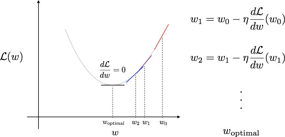
Since we don’t know where this is to begin with, we start with a guess at any point $w_0$. And then we feel around our local neighbourhood and head in the downward direction of the slope. This gets us to the point $w_1$. Where we do this again, arriving at $w_2$. And again and again, until we reach a point where we can’t go any lower or the slope is 0. This is when we’ve found $w_{\mathrm{optimal}}$.

This is shown in the equations alongside the figure, where we’ve now introduced a parameter called the learning rate, $\eta$. This is a measure of how fast we modify our weights and is something that we need to carefully tune in practice.

The actual mechanism for finding these slopes (or gradients when we have multiple parameters) comes out of the box in TensorFlow as we’re soon going to see. But if you’re interested in the details of how this is done, you should go read about something called backward mode automatic differentiation.

Notebook 1: A linear classifier for the MNIST handwritten digit dataset in TensorFlow

Finally we have all the pieces to make our first complete learning image classifier! Given some image as a raw array of numbers, we have a parameterised score function (linear transformation followed by a softmax function) that takes us to category scores. We have a way of evaluating its performance (the cross entropy loss function). We also have an algorithm to learn from example data and improve the classifier’s parameters (optimisation via stochastic gradient descent).

So let’s pause on the theory for a bit to go work out our first practical example in the form of an IPython notebook. This example reproduces and expands upon the MNIST digit classification tutorial on the TensorFlow website aimed at beginners to machine learning. Working through this example will ensure that you have TensorFlow running properly on your machine, and allows you to experience coding up an image classifier to see all the pieces we talked about in action.

Note that all the embedded code in this article also exists as a standalone GitHub repository as a collection of iPython notebooks. Apart from having all the code in one convenient place for you to play with and extend, the repository also contains setup notes on how to get started with the code. So do fetch a copy and experiment alongside reading this article, it’ll really help solidify concepts.

With that, let’s start by importing some packages we need.

import tensorflow as tf
from tensorflow.examples.tutorials.mnist import input_data

import matplotlib.pyplot as plt
%matplotlib inline
plt.rcParams['figure.figsize'] = (5.0, 4.0)
plt.rcParams['image.cmap'] = 'Greys'

import numpy as np
np.set_printoptions(suppress=True)
np.set_printoptions(precision=2)

Getting a feel for the data

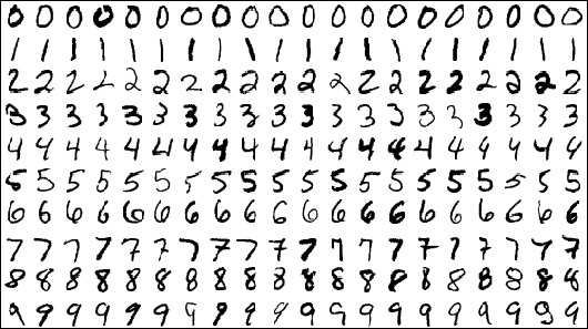
MNIST is a dataset that contains 70,000 labelled images of handwritten digits that look like the following.

We’re going to train a linear classifier on a part of this dataset, and test it against another portion of the dataset to see how well we did.

The TensorFlow tutorial comes with a handy loader for this dataset.

mnist = input_data.read_data_sets("MNIST_data/", one_hot=True)

Extracting MNIST_data/train-images-idx3-ubyte.gz
Extracting MNIST_data/train-labels-idx1-ubyte.gz
Extracting MNIST_data/t10k-images-idx3-ubyte.gz
Extracting MNIST_data/t10k-labels-idx1-ubyte.gz

The loader even handily splits the dataset into three parts:

• A training set (55000 examples) used to train the model
• A validation set (5000 examples) used to optimise hyperparameters. This is not discussed or used in this article.
• A test set (10000 examples) used to gauge the accuracy of the trained model

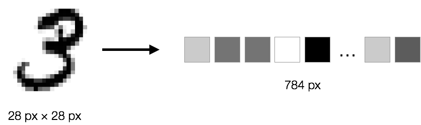
The images are greyscale and each 28 pixels wide by 28 pixels tall, and this is stored as an array of length 784.

The labels are a one hot vector of length 10, meaning it is a vector of all zeros except at the location that corresponds to the label it’s referring to. E.g. An image with a label 3 will be represented as (0, 0, 0, 1, 0, 0, 0, 0, 0, 0).

print mnist.train.images.shape
print mnist.train.labels.shape

(55000, 784)
(55000, 10)

print mnist.test.images.shape
print mnist.test.labels.shape

(10000, 784)
(10000, 10)

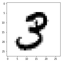
We can get a better sense for one of these examples by visualising the image and looking at the label.

example_image = mnist.train.images[1]
example_image_reshaped = example_image.reshape((28, 28)) # Can't render a line of 784 numbers
example_label = mnist.train.labels[1]

print example_label
plt.imshow(example_image_reshaped)

[ 0.  0.  0.  1.  0.  0.  0.  0.  0.  0.]

Setting up a score function, loss function and optimisation algorithm

Now that we have a better sense of the dataset we’re working with, let’s move onto the machine learning bits.

First, we setup some placeholders to hold batches of this training data for when we learn our model. The reason why we work in batches is that it’s easier on memory than holding the entire set. And it’s this notion of working with (random) batches of input rather than the entire set that moves us from the realm of Gradient Descent that we saw earlier, to Stochastic Gradient Descent that we have here.

x = tf.placeholder(tf.float32, [None, 784])
y_ = tf.placeholder(tf.float32, [None, 10])

We define our linear model for the score function after introducing two of parameters, W and b.

W = tf.Variable(tf.zeros([784, 10]))
b = tf.Variable(tf.zeros([10]))
y = tf.nn.softmax(tf.matmul(x, W) + b)

We define our loss function to measure how poorly this model performs on images with known labels. We use the a specific form called the cross entropy loss.

cross_entropy = tf.reduce_mean(-tf.reduce_sum(y_*tf.log(y), reduction_indices=[1]))

Using the magic of blackbox optimisation algorithms provided by TensorFlow, we can define a single step of the stochastic gradient descent optimiser (to improve our parameters for our score function and reduce the loss) in one line of code.

train_step = tf.train.GradientDescentOptimizer(0.5).minimize(cross_entropy)

Training the model

The way TensorFlow works, we haven’t really executed any of the code above in the classic sense. All we’ve done is defined what’s called the computational graph.

Now we go ahead and initialise a session to actually train the model and evaluate its performance.

init = tf.global_variables_initializer()
sess = tf.Session()
sess.run(init)

We train the model iteratively for 1000 steps, loading a batch of example images each time.

for i in range(1000):
  batch_xs, batch_ys = mnist.train.next_batch(100)
  sess.run(train_step, feed_dict={x: batch_xs, y_: batch_ys})

Verifying the results

At this point, our model is trained. And we can deterime in the accuracy by passing in all the test images and labels, figuring out our own labels, and averaging out the results.

correct_prediction = tf.equal(tf.argmax(y, 1), tf.argmax(y_, 1))
accuracy = tf.reduce_mean(tf.cast(correct_prediction, tf.float32))
print(sess.run(accuracy, feed_dict={x: mnist.test.images, y_: mnist.test.labels}))

0.9205

Around 92%, that’s pretty good!

Moving to neural networks

The linear image classifier we just built works surprisingly well for the MNIST digit dataset (around 92% accurate). I think this is pretty amazing, because what this implies is that these images are (mostly) linearly separable in the 784 dimensional space that they’re represented in. Meaning you can draw 10 lines ($n-1$ dimensional hyperplanes, really) in a plane ($n$ dimensional space, really) with these digits and neatly separate them into categories.

But if you read the TensorFlow tutorial that deals with the same dataset, they explicitly point out that:

“Getting 92% accuracy on MNIST is bad. It’s almost embarrassingly bad.”

So if you’re like the author of this tutorial and want to improve the performance of our classifier (or handle a more general dataset beyond neatly normalised greyscale digits) we need to move to a more general, nonlinear score function. The cool thing is that as we generalise the score function, the rest of the machinery (the loss function and optimisation process) stays the same!

Making the score function nonlinear

To make the score function nonlinear, we first introduce what’s called a neuron. This is the simple function shown in the following animation that does three things:

1. It multiplies each of its inputs by a weight.
2. It sums these weighted inputs to a single number and adds a bias.
3. It passes this number through a nonlinear function called the activation and produces an output.

These neurons can be arranged into layers to form a neural network that on the outer layers match the shape of our input and our output. For the MNIST dataset that we’ve been working with, this is a vector of 784 numbers coming in and 10 numbers going out. The layer in the middle is called the hidden layer since we don’t directly access it on the input or the output. It can be of arbitrary size, and this is the sort of thing that defines the architecture of the network. In neural network parlance the network shown below is called a two layer network or a one hidden layer network. (We can have as many of these hidden layers as we need.)

By stacking neurons in this fashion, we can express in a straightforward manner the operations performed by the network in matrix-vector notation:

1. It takes in an input vector $\mathbf{x}$.
2. The hidden layer first performs a linear operation with some weights and biases, $$ \mathbf{y}_1 = \mathbf{W}_1 \mathbf{x} + \mathbf{b}_1, $$ followed by the simplest possible nonlinearity we can imagine, a piece-wise linear function called rectified linear unit (ReLU): $$ \mathbf{h}_1 = \max(0, \mathbf{y}_1). $$ (There are many other functional forms one could use for this nonlinear activation function, but this one form is really popular todayand will suffice for our needs.)
3. Finally we stack an additional matrix-vector linear operation (introducing another set of weights and biases) to bring our output back to the size we want, 10 numbers going out. $$ \mathbf{y}_2 = \mathbf{W}_2 \mathbf{h}_1 + \mathbf{b}_2 $$ As before, we pass this output through a softmax function $\sigma$ so that we an interpret the output as the probability of each category. $$ \mathbf{s} = \sigma(\mathbf{y}_2) $$

And that’s all there is really to neural networks. If you stare at them closely, you’ll see that they’re just collections of matrix multiplications interwoven with element-wise nonlinear activation functions.

Notebooks 2 & 3: A neural network-based MNIST digit classifier in TensorFlow

If you start digging into neural network theory, you’ll stumble across the fact that the one hidden layer network architecture we just introduced can approximate any functional form. Now, much like the fact that the linear classifier worked at all, this seems like a mind-blowing result. But if you look at the proofs for this a bit closer you’ll realise that they cheat with having as many neurons as they need in the hidden layer. Because then you can apply Weierstrass approximation theorem or whatever and you’re done.

We’ll spend some time later getting a better feeling for the representative power of neural networks in general, but for now, let’s pause with theory and return to our practical example. We’re going to extend our linear image classifier to one based on a neural network, and hopefully see amazing gains in classification accuracy in the process!

The code for this extension is developed across two new notebooks in the accompanying repository: Notebook 2 and Notebook 3. Since the actual code changes relative to the linear classifier are minimal (we’re only replacing the score function with a nonlinear version after all), I’m only going to step through the differences and their implications in what follows. Feel free to go through the notebooks in their entirety if you would like more context.

Recall that in the linear case we saw previously, the model for the score function was:

W = tf.Variable(tf.zeros([784, 10]))
b = tf.Variable(tf.zeros([10]))
y = tf.nn.softmax(tf.matmul(x, W) + b)

Now we redefine this to be a nonlinear model with a few additional lines of code. Our new model is the one hidden layer network architecture we saw earlier. This introduces two sets of parameters: W1, b1 and W2, b2 that we need to learn.

W1 = tf.Variable(tf.zeros([784, 100]))
b1 = tf.Variable(tf.zeros([100]))
h1 = tf.nn.relu(tf.matmul(x, W1) + b1)

W2 = tf.Variable(tf.zeros([100, 10]))
b2 = tf.Variable(tf.zeros([10]))
y = tf.nn.softmax(tf.matmul(h1, W2) + b2)

As before, we then define the cross entropy loss function that quantifies how poorly his model performs on images with known labels and use the stochastic gradient descent optimiser to iteratively improve parameters and minimise the loss. And once this model is trained, we can pass it test images and labels and determine the average accuracy.

correct_prediction = tf.equal(tf.argmax(y, 1), tf.argmax(y_, 1))
accuracy = tf.reduce_mean(tf.cast(correct_prediction, tf.float32))
print(sess.run(accuracy, feed_dict={x: mnist.test.images, y_: mnist.test.labels}))

0.1135

11%?!? We expected to see amazing gains over 92% in our accuracy, but instead see something terrible. Why? Why after all this talk of universal approximators is our outcome so poor?

It turns out that just because our score function can theoretically fit anything doesn’t mean our learning algorithm can always find this fit. And if you look at the model definition code above from Notebook 2, you’ll realise that this is because we initialised all our weights and biases to 0. And it just so happens that because of the way ReLUs are defined, starting everything at 0 means that they’re dead (or don’t fire) from the get-go, and gradient descent can’t really modify and improve upon the parameters.

This explains the output of 10—11% accuracy, which is basically what you’d get if you guessed at random between 10 possible categories. So what we need to do is to improve the initialisation of these parameters as we’ve done in Notebook 3.

W1 = tf.Variable(tf.truncated_normal(shape=[784, 100], stddev=0.1))
b1 = tf.Variable(tf.constant(0.1, shape=[100]))
h1 = tf.nn.relu(tf.matmul(x, W1) + b1)

W2 = tf.Variable(tf.truncated_normal(shape=[100, 10], stddev=0.1))
b2 = tf.Variable(tf.constant(0.1, shape=[10]))
y = tf.nn.softmax(tf.matmul(h1, W2) + b2)

We initialise the weights with truncated normals (literally picking values from a normal distribution that’s been truncated to within two standard deviations around the mean) and initialise biases to a small positive constant, 0.1.

With this seemingly trivial change, retraining the model and verifying its average accuracy on the test data tells a very different story.

correct_prediction = tf.equal(tf.argmax(y, 1), tf.argmax(y_, 1))
accuracy = tf.reduce_mean(tf.cast(correct_prediction, tf.float32))
print(sess.run(accuracy, feed_dict={x: mnist.test.images, y_: mnist.test.labels}))

0.9654

Over 96% accurate! Much better.

And finally, convolutional neural networks

We’re in a really good place right now in terms of our understanding and capability. We’ve managed to build a (two-layer) neural network that does an excellent job of classifying images. (Over 96% on the MNIST data.) You would’ve also noticed that this extension didn’t take too much more code than the linear classifier we built initially.

If I were to ask you now how we could further improve the accuracy of our classifier, you’d probably point out that this is easy to do by adding more layers to our score function (i.e. making our model deeper). Perhaps something like the following:

TODO: Insert somewhere around here the story about using the TensorFlow playground to get a feeling for the representative power of neural nets. That they can automatically learn features we’d need to otherwise hand engineer.

The intuition being that even though each neuron is barely nonlinear, introducing more layers of them allows for more nonlinearity, increasing the approximation capability of the score function. While this is indeed true, there are some fundamental drawbacks with the general form of neural networks we’ve seen so far (the term for them is standard or fully-connected neural networks):

Firstly, they entirely disregard the 2D structure of the image at the get-go. Remember that instead of working with the input as $28 \times 28$ matrix, they worked with the input as a 784 number array. And you can imagine there is some useful information in pixels sharing proximity that’s being lost.

Secondly, the number of parameters we would need to learn grows really rapidly as we add more layers. Here are the number of parameters corresponding to the examples we’ve seen so far:

• Linear: 784*10 + 10 = 7,850
• Neural network (one hidden layer): 784100 + 100 + 10010 + 10 = 79,510
• Neural network (two hidden layers): 784400 + 400 + 400100 + 100 + 100*10 + 10 = 355,110

The fundamental reason for this rapid growth in parameters is that every neuron in a given layer sees all neurons in the previous layer. Furthermore, you can imagine how much worse this would be if our input image wasn’t tiny (28 px $\times$ 28 px) but instead more realistically sized.

Convolutional neural networks (convnets) are architected to solve both these issues, making them particularly powerful for dealing with image data. And we’ll soon see how we can use them to build a deep image classifier that’s state of the art.

Architecture of convnets in general

Convnets are very similar to fully-connected neural networks in that they’re made up of neurons arranged in layers and they have learnable weights and biases. Each neuron receives some inputs, does a linear map and optionally follows it with a nonlinear activation. The whole network still expresses a single score function: from the raw image pixels on one end to class scores at the other.

The thing that makes convnets special is that they make the explicit assumptions on the structure of the input, in our case images, that allow them to encode certain nice properties in their architecture. These choices make them efficient to implement and vastly reduce the amount of parameters in the network as we’ll soon see.

TODO: Figure of the differences between standard and convolutional neural networks.

Instead of dealing with the input data (and arranging intermediate layers of neurons) as linear arrays, they deal with information as 3D volumes (with width, height and depth). i.e. Every layer takes as input a 3D volume of numbers and outputs a 3D volume of numbers. What one imagines as a 2D input image ($W \times H$) gets transformed into 3D by introducing the colour depth as the third dimension ($W \times H \times d$). (Recall that this for the MNIST digit data would be 1 because it’s greyscale, but for a colour RGB image the depth would be 3.) Similarly what one might imagine as a linear output of length $C$ is actually represented as $1 \times 1 \times C$.

Convnets do this with the help of two different layer types.

Convolutional (Conv) layer

The first is the convolutional (Conv) layer, and you can think of it as a set of learnable filters. Let’s say we have $K$ such filters. Each filter is small spatially, with an extent denoted by $F$, but extends to the depth of its input. e.g. A typical filter might be $3 \times 3 \times 3$ ($F = 3$ pixels wide and high, and $3$ from the depth of the input 3-channel colour image).

Now we slide or convolve this filter set over the input volume (with a stride $S$ that denotes how fast we move). This input can be spatially padded ($P$) with zeros as needed for controlling output spatial dimensions. As we slide, each filter computes a sort of volumetric dot product with the input to produce a 2D output, and when we stack these across all the filters we have in our set, we get a 3D output volume.

This is going to take you a bit of time to think about and process, but the idea is quite simple when you get it.

The interesting things to note here are that:

1. Because this filter set is the same as we vary spatial position, once they’ve learnt to get excited about a feature, say a slanted line in one position, they’ve learnt to get excited at any spatial position. i.e. Translation of features around the input image doesn’t matter.

2. We’re no longer ballooning in terms of number of parameters even if the input image size grows a lot or our number of layers grow. All we need to learn are the weights and biases that correspond to our sets of filters (denoted in red in the animation above), which are particularly small in number because of their small spatial size.

Pooling (Pool) layer

The second important kind of layer in convnets is the pooling (Pool) layer. This is much easier to understand, as it simply acts as a downsampling filter. These are used to reduce computational cost, and to some extent also reduce overfitting. Note that it has no parameters to learn!

TODO: Depict a pool layer in a figure.

For example, a max pooling layer with a spatial extent $F = 2$ and a stride $S = 2$ halves the input spatial dimension from $4 \times 4$ to $2 \times 2$, leaving the depth unchanged. It does this by picking the maximum of each set of $2 \times 2$ numbers and passing only those along to the output. You have one such pooling layer for each input depth slice to cover the entire input volume.

You can also do average pooling and other kinds of downsampling.

Notebook 4: A convnet-based MNIST digit classifier in TensorFlow

Now that we’ve taken a theoretical look at the two kinds of layers that are core to convnets (Conv and Pool), we’re going to get a better feeling for them by using them in a practical example. Let’s return to extend our MNIST digit classifier with these additional two layers and see what kinds of gains we get in classification accuracy.

This example is a simplification of Deep MNIST for Experts tutorial on the TensorFlow website. And as before, the complete code for this example lives in a standalone notebook in the accompanying repository. Here I only step through the differences relative to our earlier (fully-connected) neural network version.

Before we get to the code, let’s reintroduce some abstract notation to better explain the changes we’re making.

FC = Fully Connected Layer
Softmax = Softmax Layer
ReLU = Rectified Linear Unit Activation
Conv = Convolutional Layer
Pool = Pool Layer

Using this notation, the models we’ve used for the score function so far are:

1. Linear: FC -> Softmax
2. Neural network (one hidden layer): FC -> ReLU -> FC -> Softmax

And the convnet-based model we’re going to setup using the code below is:

Conv -> ReLU -> Pool -> FC -> ReLU -> FC -> Softmax

# Define some helper functions to ease the definition of the model
def weight_variable(shape):
    return tf.Variable(tf.truncated_normal(shape, stddev=0.1))

def bias_variable(shape):
    return tf.Variable(tf.constant(0.1, shape=shape))

def conv(x, W):
    return tf.nn.conv2d(x, W, strides=[1, 1, 1, 1], padding='SAME')

def pool(x):
    return tf.nn.max_pool(x, ksize=[1, 2, 2, 1], strides=[1, 2, 2, 1], padding='SAME')

# A score function (model) composed of a few layers

# Reshape the input to look like a volume (Input)
x_image = tf.reshape(x, [-1, 28, 28, 1])

# A convolutional layer (CONV -> RELU -> POOL)
W_conv = weight_variable([5, 5, 1, 32])
b_conv = bias_variable([32])
h_conv = tf.nn.relu(conv(x_image, W_conv) + b_conv)
h_pool = pool(h_conv)

# A densely connected layer (FC)
W_fc1 = weight_variable([14*14*32, 1024])
b_fc1 = bias_variable([1024])
h_pool_flat = tf.reshape(h_pool, [-1, 14*14*32])
h_fc1 = tf.nn.relu(tf.matmul(h_pool_flat, W_fc1) + b_fc1)

# Another densely connected layer (for "readout") (FC)
W_fc2 = weight_variable([1024, 10])
b_fc2 = bias_variable([10])
y = tf.nn.softmax(tf.matmul(h_fc1, W_fc2) + b_fc2)

As before, we then define the cross entropy loss function that quantifies how poorly this model performs on images with known labels and use an optimiser to iteratively improve parameters and minimise the loss. And once this model is trained, we can pass it test images and labels and determine the average accuracy.

print(sess.run(accuracy, feed_dict={x: mnist.test.images, y_: mnist.test.labels}))

0.989

Nearly 99% accurate! Great!

How do convnets work (so well)?

If you found yourself working through Notebook 4 being fuzzy about how our convnet-based classifier actually works, here is a wonderful webpage that provides more insight.

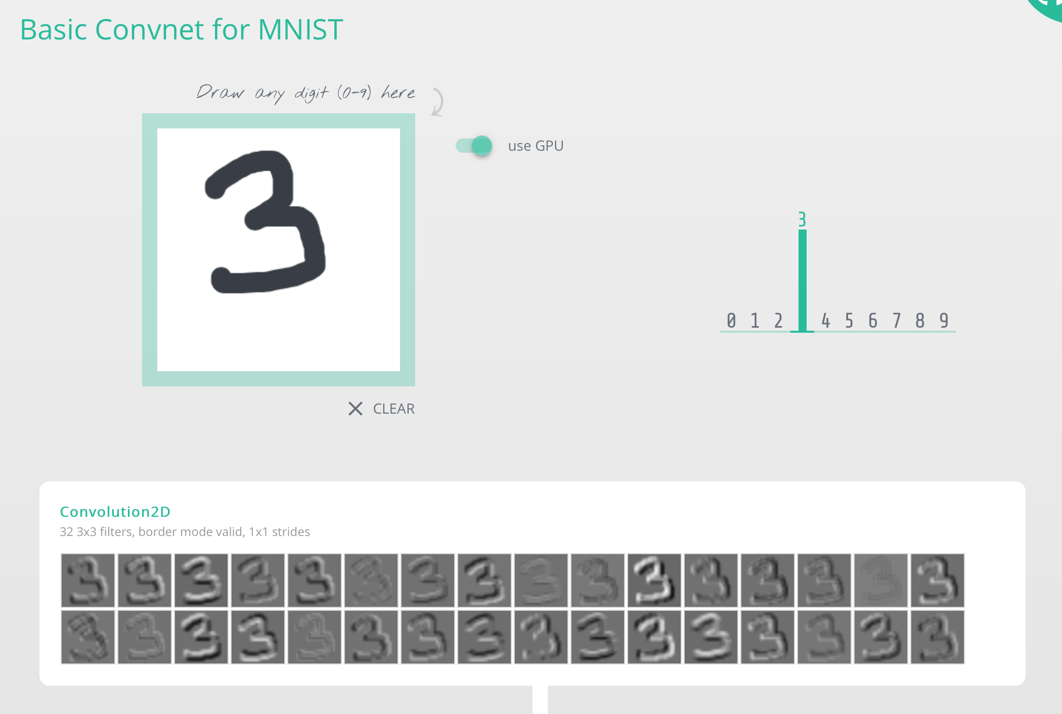
You play around with it by drawing any digit you want. As you do, the webpage helps visualise the outputs of the different layers, leading to the (softmax) classification in the end. You get a sense that as you go from layer to layer, the system essentially transforms representations of the input into forms that are more suitable to the task at hand — classification in our case.

To reiterate this, let’s look at another visualisation of a convnet classifier.

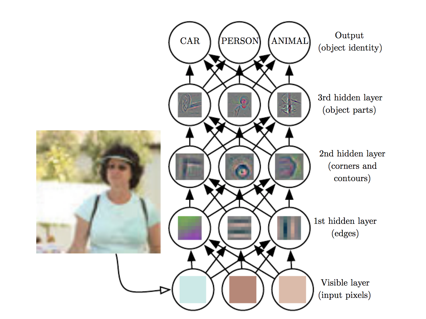
Given raw pixel input, the first hidden layer get excited by simple features like edges, the next layer perhaps things like contours, and the next maybe simple shapes and part of objects. And the deeper you go, the more they start to grasp the entire input field, not just a narrow region, but more importantly, the closer they’re moving toward a representation that makes it easy for them to classify on.

It turns out that convolutional neural networks are all about representation learning. This is what makes them so powerful.

In fact, this is true of deep learning in general (we call these models deep as we start to stack on more layers). It’s just that convnets are disproportionately used as teaching examples (as I’m doing right now) because each layer does something at least vaguely recognisable to humans.

TODO: Polish this section and connect back to the idea that we turned to machine learning in the first place because we found it so difficult to write a program that hand-engineered features for image classification.

Returning to the style transfer problem

Now that we have the vocabulary to talk about convnets and have some insight into how they behave, we’re finally in a good place to return to the original style transfer problem that motivated this entire journey.

Recall that we had a content image $\mathbf{c}$ and a style image $\mathbf{s}$, and the core of this effect was to somehow extract the style (the colour and textures) from $\mathbf{s}$ and apply it to the content (the structure) from $\mathbf{c}$ to arrive at the sort of example output shown below.

Recall also that after looking at the original paper from Gatys et al., we were able to pose this as an optimisation problem:

$$ \mathbf{x}^* = \underset{\mathbf{x}}{\operatorname{argmin}}\left(\alpha \mathcal{L}_{\mathrm{content}}(\mathbf{c}, \mathbf{x}) + \beta \mathcal{L}_{\mathrm{style}}(\mathbf{s}, \mathbf{x})\right) $$

That is, we are looking for an image $\mathbf{x}$ that differs as little as possible in terms of content from the content image $\mathbf{c}$, while simultaneously differing as little as possible in terms of style from the style image $\mathbf{s}$. The only hitch in this plan was that we didn’t have a convenient way to gauge the differences between images in terms of content and style.

But now we do!

It turns out that convnets pre-trained for image classification have already learnt to encode perceptual and semantic information that we need to measure these semantic difference terms! The primary explanation for this is that when learning object recognition, the network has to become invariant to all image variation that’s superfluous to object identity.

So in what follows, we’re first going to get acquainted with a particular deep convnet-based image classifier called VGGNet, and soon see how it can be repurposed for the style transfer problem.

The convnet-based classifier at the heart of the Gatys paper

When we completed Notebook 4, we’d worked out a simple convnet-based image classifier that did a great job at classifying the MNIST dataset. Now we’re going to see a family of more powerful architectures called VGGNet that can work with more general data: colour images of different objects. This network is at the core of the Gatys style transfer paper as we’ll soon see.

Recall that when we last implemented even our simple convnet, it was hard to write (in terms of boilerplate code, and keeping careful track of the shapes of the objects flowing through the code) and slow to train. To circumvent that, we aren’t going to write VGGNet from scratch. We’re going to instead use a version that someone else has already written and pre-trained.

To simplify our lives even further, we’re no longer going to use TensorFlow proper from this point on — we’re going to move to a higher-level library called Keras. About a month ago it was announced that Keras is going to be folded into the official TensorFlow project — meaning that the simpler API you’re going to see could soon be TensorFlow’s API! This is great because TensorFlow often operates at a lower level than you care about when you want to simply quickly experiment with deep learning.

I’ve incorporated Notebook 5 in its entirety below since it is very different from the notebooks we’ve seen thus far.

Notebook 5: Fetching and playing with a pre-trained VGGNet (16) in Keras

Let’s start by importing some packages we need. Note that even though we’ve moved to Keras, it uses TensorFlow in the background for low-level operations like tensor products and convolutions.

import numpy as np
from PIL import Image

from keras.applications.vgg16 import VGG16
from keras.applications.vgg16 import preprocess_input, decode_predictions

Using TensorFlow backend.

Getting a feel for the model and data it is trained on

In this notebook, we’re going to fetch a network that is pre-trained on the ImageNet data set. In particular, we’re going to fetch the VGGNet model with 16 layers (that we’re going to refer to as VGG16).

The ImageNet project is a large visual database designed for use in visual object recognition software research. As of 2016, over ten million URLs of images have been hand-annotated by ImageNet to indicate what objects are pictured. ImageNet crowdsources its annotation process.

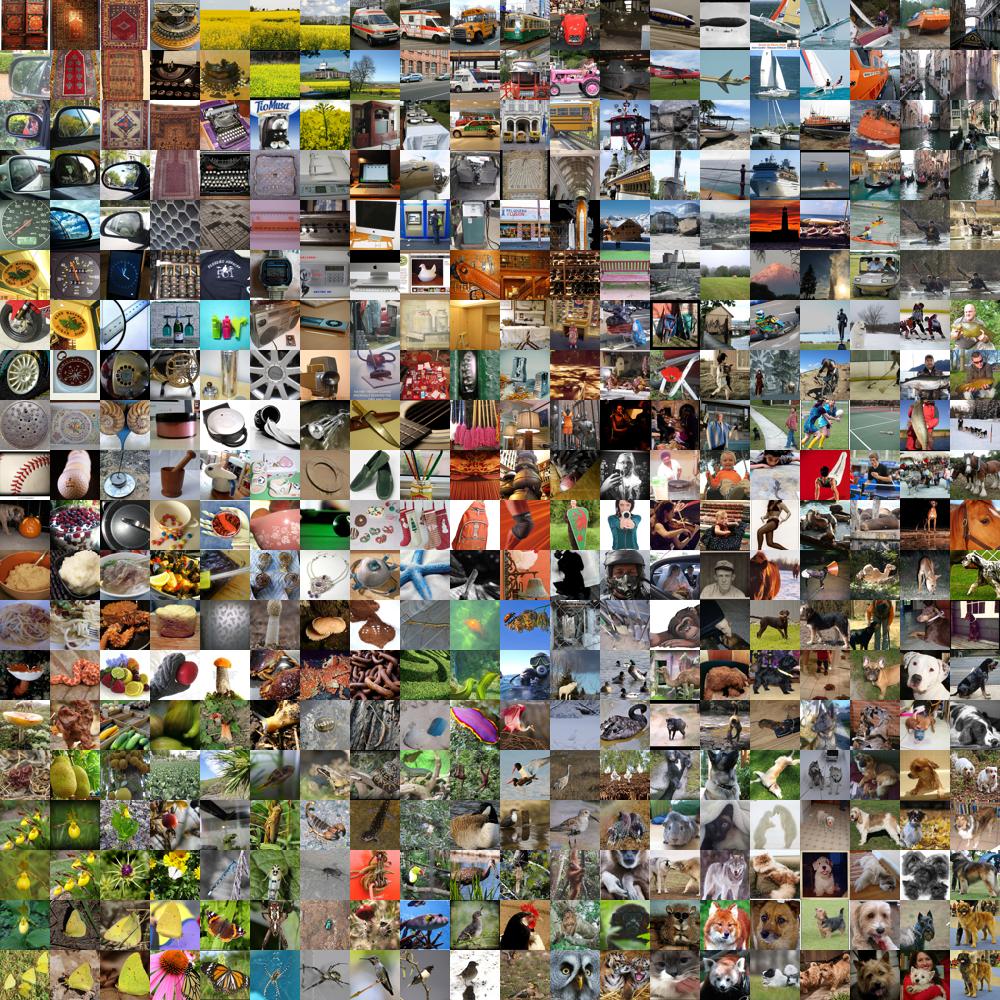
Since 2010, the annual ImageNet Large Scale Visual Recognition Challenge (ILSVRC) is a competition where research teams submit programs that classify and detect objects and scenes. (This is like the Olympics of computer vision challenges!)

VGGNet was introduced as one of the contenders in 2014’s ImageNet Challenge and secured the first and the second places in the localisation and classification tracks respectively. It was later described in great detail in a paper that came out the following year. The paper describes how a family of models essentially composed of simple ($3 \times 3$) convolutional filters with increasing depth (11–19 layers) managed to perform so well at a range of computer vision tasks.

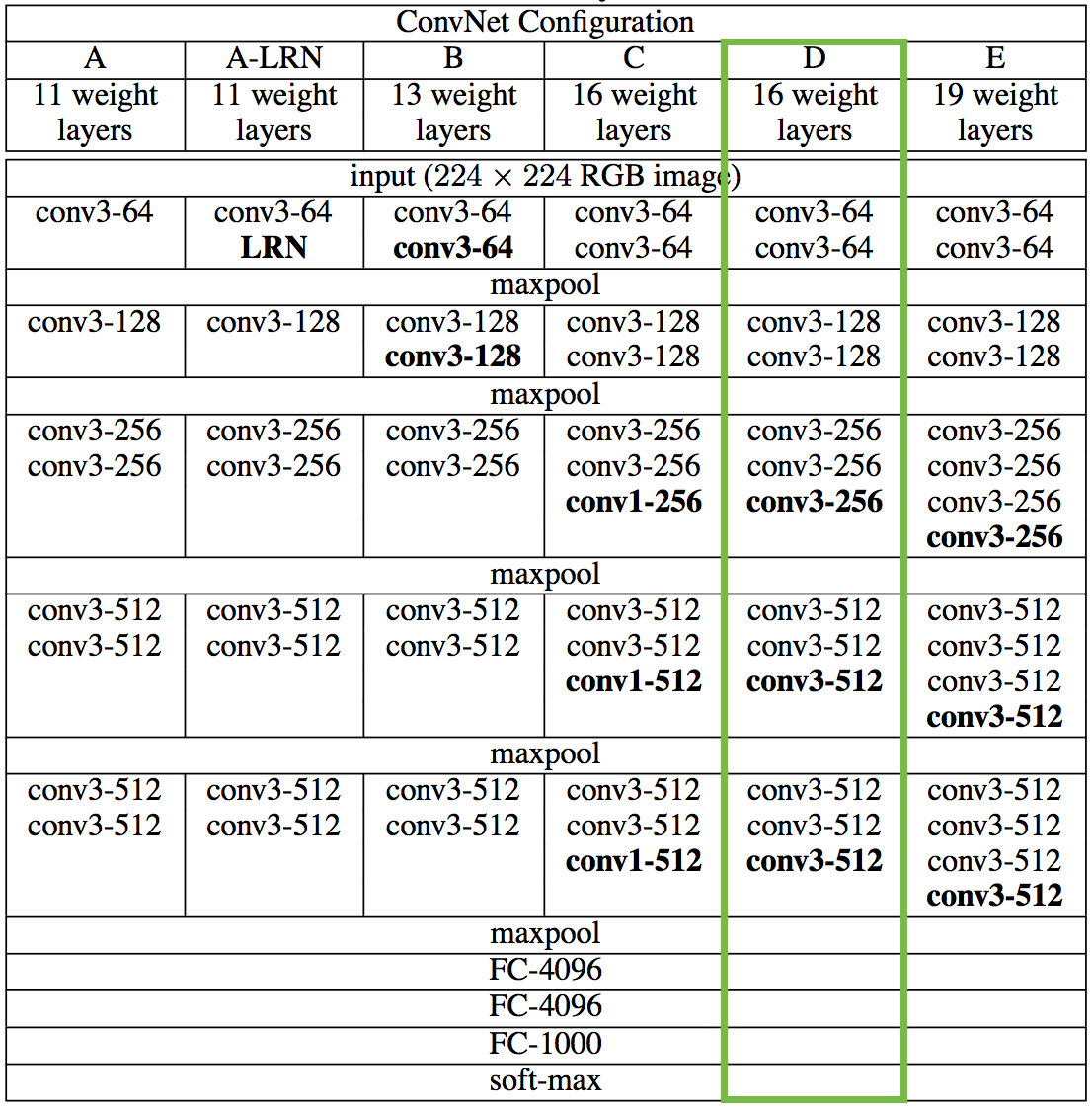
We’re going to first reproduce the 16 layer variant marked in green for classification, and in the next notebook we’ll see how it can be repurposed for the style transfer problem.

Fetching a pretrained model in Keras

This is trivial to do in Keras, and can be done in a single line. There is a selection of such models one can import.

model = VGG16(weights='imagenet', include_top=True)

Let’s take a look at the model, convince ourselves it looks the same as the paper.

layers = dict([(layer.name, layer.output) for layer in model.layers])
layers

{'block1_conv1': <tf.Tensor 'Relu:0' shape=(?, 224, 224, 64) dtype=float32>,
 'block1_conv2': <tf.Tensor 'Relu_1:0' shape=(?, 224, 224, 64) dtype=float32>,
 'block1_pool': <tf.Tensor 'MaxPool:0' shape=(?, 112, 112, 64) dtype=float32>,
 'block2_conv1': <tf.Tensor 'Relu_2:0' shape=(?, 112, 112, 128) dtype=float32>,
 'block2_conv2': <tf.Tensor 'Relu_3:0' shape=(?, 112, 112, 128) dtype=float32>,
 'block2_pool': <tf.Tensor 'MaxPool_1:0' shape=(?, 56, 56, 128) dtype=float32>,
 'block3_conv1': <tf.Tensor 'Relu_4:0' shape=(?, 56, 56, 256) dtype=float32>,
 'block3_conv2': <tf.Tensor 'Relu_5:0' shape=(?, 56, 56, 256) dtype=float32>,
 'block3_conv3': <tf.Tensor 'Relu_6:0' shape=(?, 56, 56, 256) dtype=float32>,
 'block3_pool': <tf.Tensor 'MaxPool_2:0' shape=(?, 28, 28, 256) dtype=float32>,
 'block4_conv1': <tf.Tensor 'Relu_7:0' shape=(?, 28, 28, 512) dtype=float32>,
 'block4_conv2': <tf.Tensor 'Relu_8:0' shape=(?, 28, 28, 512) dtype=float32>,
 'block4_conv3': <tf.Tensor 'Relu_9:0' shape=(?, 28, 28, 512) dtype=float32>,
 'block4_pool': <tf.Tensor 'MaxPool_3:0' shape=(?, 14, 14, 512) dtype=float32>,
 'block5_conv1': <tf.Tensor 'Relu_10:0' shape=(?, 14, 14, 512) dtype=float32>,
 'block5_conv2': <tf.Tensor 'Relu_11:0' shape=(?, 14, 14, 512) dtype=float32>,
 'block5_conv3': <tf.Tensor 'Relu_12:0' shape=(?, 14, 14, 512) dtype=float32>,
 'block5_pool': <tf.Tensor 'MaxPool_4:0' shape=(?, 7, 7, 512) dtype=float32>,
 'fc1': <tf.Tensor 'Relu_13:0' shape=(?, 4096) dtype=float32>,
 'fc2': <tf.Tensor 'Relu_14:0' shape=(?, 4096) dtype=float32>,
 'flatten': <tf.Tensor 'Reshape_13:0' shape=(?, ?) dtype=float32>,
 'input_1': <tf.Tensor 'input_1:0' shape=(?, 224, 224, 3) dtype=float32>,
 'predictions': <tf.Tensor 'Softmax:0' shape=(?, 1000) dtype=float32>}

Looks good. And we now let’s get a sense for how many parameters they are in this model.

model.count_params()

138357544

Woah, that’s a lot! We’ve just gotten around needing to train a model containing 138+ million parameters.

Using it for classification

Now that we have our pre-trained model loaded, we can use it for classification.

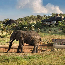
Load an test image and preprocess it

image_path = 'images/elephant.jpg'
image = Image.open(image_path)
image = image.resize((224, 224))
image

# Convert it into an array
x = np.asarray(image, dtype='float32')
# Convert it into a list of arrays
x = np.expand_dims(x, axis=0)
# Pre-process the input to match the training data
x = preprocess_input(x)

Classify the test image

The following code classifies the test image and decodes the results into a list of tuples (class, description, probability). There is one such list for each sample in the batch, but since we’re only sending in one test image we only get one set of output.

preds = model.predict(x)
print('Predicted:', decode_predictions(preds, top=3)[0])

('Predicted:', [(u'n02504458', u'African_elephant', 0.84805286), (u'n01871265', u'tusker', 0.10270286), (u'n02504013', u'Indian_elephant', 0.049056333)])

The artistic style transfer algorithm

In the process of learning how to classify images, the VGG16 model that we just downloaded and played with (in Notebook 5) has actually learnt a lot more. As it has trained itself to transform the raw input pixels into category scores, it has learnt to encode quite a bit of perceptual and semantic information about images. The neural style algorithm introduced in Gatys et al. (2015) plays with these representations to first define the semantic loss terms ($\mathcal{L}_{\mathrm{content}}(\mathbf{c}, \mathbf{x})$ and $\mathcal{L}_{\mathrm{style}}(\mathbf{s}, \mathbf{x})$) and then uses these terms to pose the optimisation problem for style transfer.

TODO: Fill out this section with the following notes, incorporating whatever theory that is not covered inline in the final notebook. This corresponds to slides 37–39 of the talk.

• Summarise the Gatys, et al. paper for the core ideas (and a sketch of the solution methodology):
  • Higher layers in the network capture the high-level content in terms of objects and their arrangement in the input image but do not constrain the exact pixel values of the reconstruction. To obtain a representation of the style of an input image, we employ correlations between the different filter responses over the spatial extent of the feature maps.
  • The representations of style and content in CNNs are separable.
  • The images are synthesised by finding an image that simultaneously matches the content representation of the photograph and the style representation of the respective piece of art.
  • Based on VGG16 - 3 FC layers. Normal VGG takes an image and returns a category score, but Gatys instead take the outputs at intermediate layers and construct L_content and L_style.
  • A figure showing off the algorithm.
• Additional technicalities: Introduce L-BFGS as a valid quasi-Newton approach to solve the optimisation problem.

Notebook 6: Concrete implementation of the artistic style transfer algorithm

Since Gatys et al. (2015) is a very exciting paper, there exist many open source implementations of the algorithm online. One of the most popular and general purpose ones is by Justin Johnson and implemented in Torch. I’ve instead followed a simple example in Keras and expanded into a fully-fledged notebook that explains many details step by step. I’ve reproduced it below in its entirety.

As always, we start with importing some packages we need. Note that we don’t require too many packages.

from __future__ import print_function

import time
from PIL import Image
import numpy as np

from keras import backend
from keras.models import Model
from keras.applications.vgg16 import VGG16

from scipy.optimize import fmin_l_bfgs_b
from scipy.misc import imsave

Using TensorFlow backend.

Load and preprocess the content and style images

Our first task is to load the content and style images. Note that the content image we’re working with is not particularly high quality, but the output we’ll arrive at the end of this process still looks really good.

height = 512
width = 512

content_image_path = 'images/hugo.jpg'
content_image = Image.open(content_image_path)
content_image = content_image.resize((width, height))
content_image

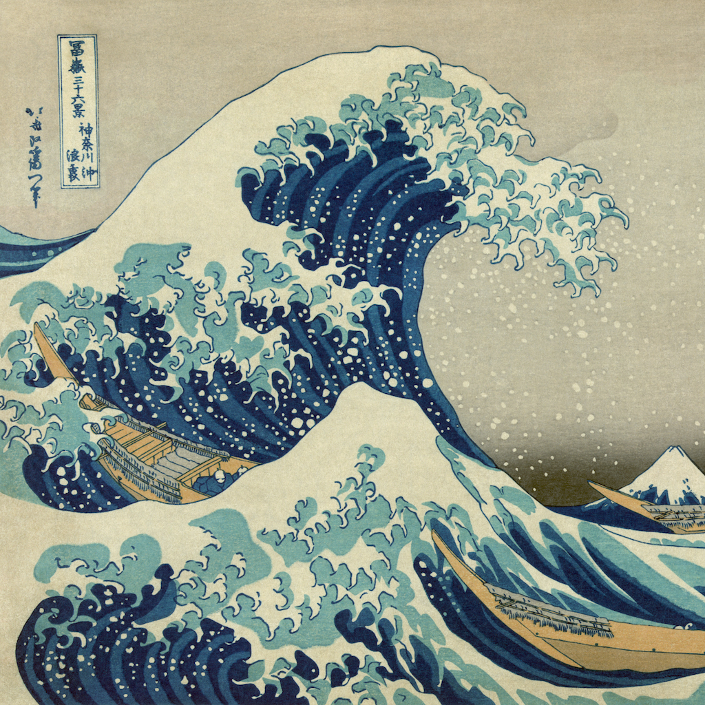
style_image_path = 'images/styles/wave.jpg'
style_image = Image.open(style_image_path)
style_image = style_image.resize((width, height))
style_image

Then, we convert these images into a form suitable for numerical processing. In particular, we add another dimension (beyond the classic height x width x 3 dimensions) so that we can later concatenate the representations of these two images into a common data structure.

content_array = np.asarray(content_image, dtype='float32')
content_array = np.expand_dims(content_array, axis=0)
print(content_array.shape)

style_array = np.asarray(style_image, dtype='float32')
style_array = np.expand_dims(style_array, axis=0)
print(style_array.shape)

(1, 512, 512, 3)
(1, 512, 512, 3)

Before we proceed much further, we need to massage this input data to match what was done in Simonyan and Zisserman (2015), the paper that introduces the VGG Network model that we’re going to use shortly.

For this, we need to perform two transformations:

1. Subtract the mean RGB value (computed previously on the ImageNet training set and easily obtainable from Google searches) from each pixel.
2. Flip the ordering of the multi-dimensional array from RGB to BGR (the ordering used in the paper).

content_array[:, :, :, 0] -= 103.939
content_array[:, :, :, 1] -= 116.779
content_array[:, :, :, 2] -= 123.68
content_array = content_array[:, :, :, ::-1]

style_array[:, :, :, 0] -= 103.939
style_array[:, :, :, 1] -= 116.779
style_array[:, :, :, 2] -= 123.68
style_array = style_array[:, :, :, ::-1]

Now we’re ready to use these arrays to define variables in Keras' backend (the TensorFlow graph). We also introduce a placeholder variable to store the combination image that retains the content of the content image while incorporating the style of the style image.

content_image = backend.variable(content_array)
style_image = backend.variable(style_array)
combination_image = backend.placeholder((1, height, width, 3))

Finally, we concatenate all this image data into a single tensor that’s suitable for processing by Keras’ VGG16 model.

input_tensor = backend.concatenate([content_image,
                                    style_image,
                                    combination_image], axis=0)

Reuse a model pre-trained for image classification to define loss functions

The core idea introduced by Gatys et al. (2015) is that convolutional neural networks (CNNs) pre-trained for image classification already know how to encode perceptual and semantic information about images. We’re going to follow their idea, and use the feature spaces provided by one such model to independently work with content and style of images.

The original paper uses the 19 layer VGG network model from Simonyan and Zisserman (2015), but we’re going to instead follow Johnson et al. (2016) and use the 16 layer model (VGG16). There is no noticeable qualitative difference in making this choice, and we gain a tiny bit in speed.

Also, since we’re not interested in the classification problem, we don’t need the fully-connected layers or the final softmax classifier. We only need the part of the model marked in green in the table below.

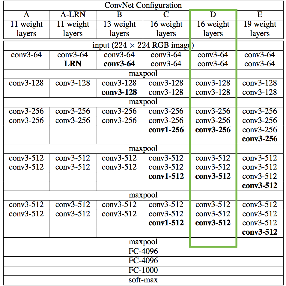
It is trivial for us to get access to this truncated model because Keras comes with a set of pretrained models, including the VGG16 model we’re interested in. Note that by setting include_top=False in the code below, we don’t include any of the fully-connected layers.

model = VGG16(input_tensor=input_tensor, weights='imagenet',
              include_top=False)

As is clear from the table above, the model we’re working with has a lot of layers. Keras has its own names for these layers. Let’s make a list of these names so that we can easily refer to individual layers later.

layers = dict([(layer.name, layer.output) for layer in model.layers])
layers

{'block1_conv1': <tf.Tensor 'Relu:0' shape=(3, 512, 512, 64) dtype=float32>,
 'block1_conv2': <tf.Tensor 'Relu_1:0' shape=(3, 512, 512, 64) dtype=float32>,
 'block1_pool': <tf.Tensor 'MaxPool:0' shape=(3, 256, 256, 64) dtype=float32>,
 'block2_conv1': <tf.Tensor 'Relu_2:0' shape=(3, 256, 256, 128) dtype=float32>,
 'block2_conv2': <tf.Tensor 'Relu_3:0' shape=(3, 256, 256, 128) dtype=float32>,
 'block2_pool': <tf.Tensor 'MaxPool_1:0' shape=(3, 128, 128, 128) dtype=float32>,
 'block3_conv1': <tf.Tensor 'Relu_4:0' shape=(3, 128, 128, 256) dtype=float32>,
 'block3_conv2': <tf.Tensor 'Relu_5:0' shape=(3, 128, 128, 256) dtype=float32>,
 'block3_conv3': <tf.Tensor 'Relu_6:0' shape=(3, 128, 128, 256) dtype=float32>,
 'block3_pool': <tf.Tensor 'MaxPool_2:0' shape=(3, 64, 64, 256) dtype=float32>,
 'block4_conv1': <tf.Tensor 'Relu_7:0' shape=(3, 64, 64, 512) dtype=float32>,
 'block4_conv2': <tf.Tensor 'Relu_8:0' shape=(3, 64, 64, 512) dtype=float32>,
 'block4_conv3': <tf.Tensor 'Relu_9:0' shape=(3, 64, 64, 512) dtype=float32>,
 'block4_pool': <tf.Tensor 'MaxPool_3:0' shape=(3, 32, 32, 512) dtype=float32>,
 'block5_conv1': <tf.Tensor 'Relu_10:0' shape=(3, 32, 32, 512) dtype=float32>,
 'block5_conv2': <tf.Tensor 'Relu_11:0' shape=(3, 32, 32, 512) dtype=float32>,
 'block5_conv3': <tf.Tensor 'Relu_12:0' shape=(3, 32, 32, 512) dtype=float32>,
 'block5_pool': <tf.Tensor 'MaxPool_4:0' shape=(3, 16, 16, 512) dtype=float32>,
 'input_1': <tf.Tensor 'concat:0' shape=(3, 512, 512, 3) dtype=float32>}

If you stare at the list above, you’ll convince yourself that we covered all items we wanted in the table (the cells marked in green). Notice also that because we provided Keras with a concrete input tensor, the various TensorFlow tensors get well-defined shapes.

The crux of the paper we’re trying to reproduce is that the style transfer problem can be posed as an optimisation problem, where the loss function we want to minimise can be decomposed into three distinct parts: the content loss, the style loss and the total variation loss.

The relative importance of these terms are determined by a set of scalar weights. These are arbitrary, but the following set have been chosen after quite a bit of experimentation to find a set that generates output that’s aesthetically pleasing to me.

content_weight = 0.025
style_weight = 5.0
total_variation_weight = 1.0

We’ll now use the feature spaces provided by specific layers of our model to define these three loss functions. We begin by initialising the total loss to 0 and adding to it in stages.

loss = backend.variable(0.)

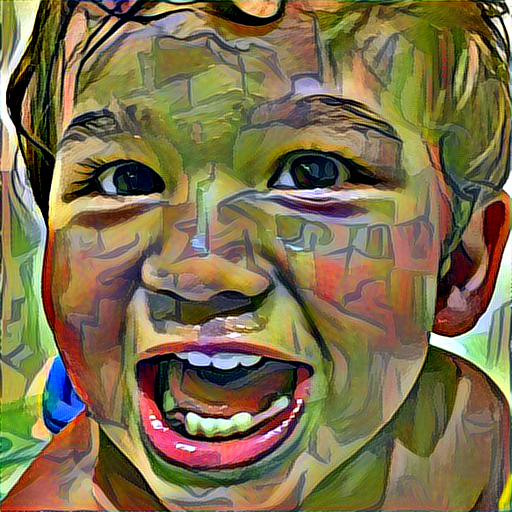
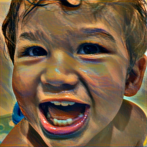
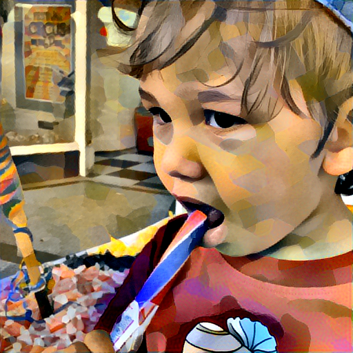
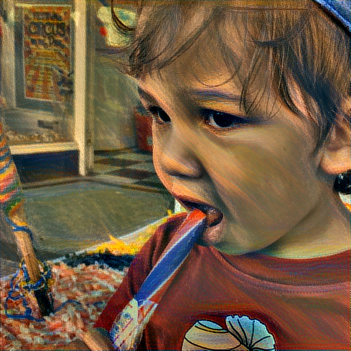
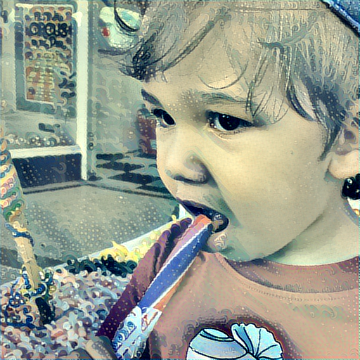
The content loss

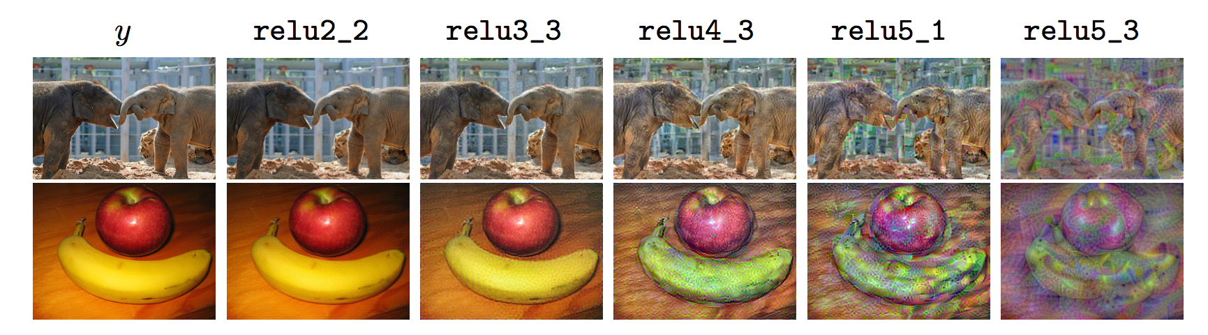
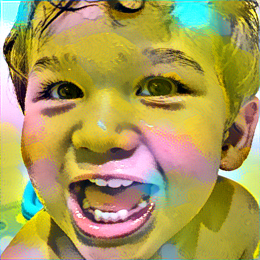
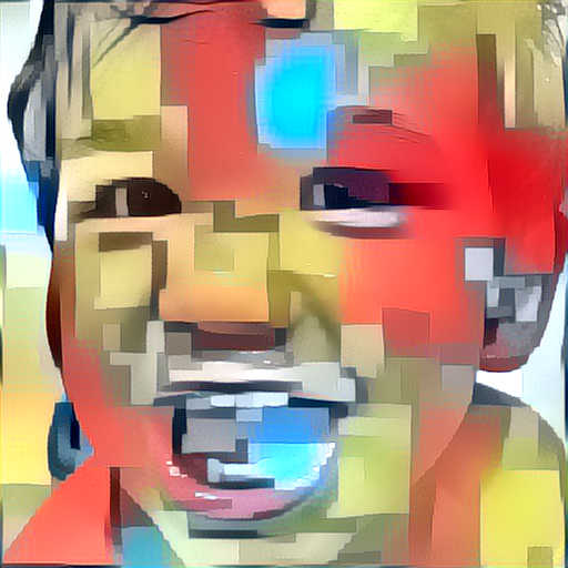
For the content loss, we follow Johnson et al. (2016) and draw the content feature from block2_conv2, because the original choice in Gatys et al. (2015) (block4_conv2) loses too much structural detail. And at least for faces, I find it more aesthetically pleasing to closely retain the structure of the original content image.

This variation across layers is shown for a couple of examples in the images below (just mentally replace reluX_Y with our Keras notation blockX_convY).

The content loss is the (scaled, squared) Euclidean distance between feature representations of the content and combination images.

def content_loss(content, combination):
    return backend.sum(backend.square(combination - content))

layer_features = layers['block2_conv2']
content_image_features = layer_features[0, :, :, :]
combination_features = layer_features[2, :, :, :]

loss += content_weight * content_loss(content_image_features,
                                      combination_features)

The style loss

This is where things start to get a bit intricate.

For the style loss, we first define something called a Gram matrix. The terms of this matrix are proportional to the covariances of corresponding sets of features, and thus captures information about which features tend to activate together. By only capturing these aggregate statistics across the image, they are blind to the specific arrangement of objects inside the image. This is what allows them to capture information about style independent of content. (This is not trivial at all, and I refer you to a paper that attempts to explain the idea.)

TODO: Make some sort of note here about the fact that the Gram matrix is a special case of a more general object. What we really want is some measure (of local-ish statistics) that’s spatially invariant.

The Gram matrix can be computed efficiently by reshaping the feature spaces suitably and taking an outer product.

def gram_matrix(x):
    features = backend.batch_flatten(backend.permute_dimensions(x, (2, 0, 1)))
    gram = backend.dot(features, backend.transpose(features))
    return gram

The style loss is then the (scaled, squared) Frobenius norm of the difference between the Gram matrices of the style and combination images.

Again, in the following code, I’ve chosen to go with the style features from layers defined in Johnson et al. (2016) rather than Gatys et al. (2015) because I find the end results more aesthetically pleasing. I encourage you to experiment with these choices to see varying results.

def style_loss(style, combination):
    S = gram_matrix(style)
    C = gram_matrix(combination)
    channels = 3
    size = height * width
    return backend.sum(backend.square(S - C)) / (4. * (channels ** 2) * (size ** 2))

feature_layers = ['block1_conv2', 'block2_conv2',
                  'block3_conv3', 'block4_conv3',
                  'block5_conv3']
for layer_name in feature_layers:
    layer_features = layers[layer_name]
    style_features = layer_features[1, :, :, :]
    combination_features = layer_features[2, :, :, :]
    sl = style_loss(style_features, combination_features)
    loss += (style_weight / len(feature_layers)) * sl

The total variation loss

Now we’re back on simpler ground.

If you were to solve the optimisation problem with only the two loss terms we’ve introduced so far (style and content), you’ll find that the output is quite noisy. We thus add another term, called the total variation loss (a regularisation term) that encourages spatial smoothness.

You can experiment with reducing the total_variation_weight and play with the noise-level of the generated image.

def total_variation_loss(x):
    a = backend.square(x[:, :height-1, :width-1, :] - x[:, 1:, :width-1, :])
    b = backend.square(x[:, :height-1, :width-1, :] - x[:, :height-1, 1:, :])
    return backend.sum(backend.pow(a + b, 1.25))

loss += total_variation_weight * total_variation_loss(combination_image)

Define needed gradients and solve the optimisation problem

The goal of this journey was to setup an optimisation problem that aims to solve for a combination image that contains the content of the content image, while having the style of the style image. Now that we have our input images massaged and our loss function calculators in place, all we have left to do is define gradients of the total loss relative to the combination image, and use these gradients to iteratively improve upon our combination image to minimise the loss.

We start by defining the gradients.

grads = backend.gradients(loss, combination_image)

We then introduce an Evaluator class that computes loss and gradients in one pass while retrieving them via two separate functions, loss and grads. This is done because scipy.optimize requires separate functions for loss and gradients, but computing them separately would be inefficient.

outputs = [loss]
outputs += grads
f_outputs = backend.function([combination_image], outputs)

def eval_loss_and_grads(x):
    x = x.reshape((1, height, width, 3))
    outs = f_outputs([x])
    loss_value = outs[0]
    grad_values = outs[1].flatten().astype('float64')
    return loss_value, grad_values

class Evaluator(object):

    def __init__(self):
        self.loss_value = None
        self.grads_values = None

    def loss(self, x):
        assert self.loss_value is None
        loss_value, grad_values = eval_loss_and_grads(x)
        self.loss_value = loss_value
        self.grad_values = grad_values
        return self.loss_value

    def grads(self, x):
        assert self.loss_value is not None
        grad_values = np.copy(self.grad_values)
        self.loss_value = None
        self.grad_values = None
        return grad_values

evaluator = Evaluator()

Now we’re finally ready to solve our optimisation problem. This combination image begins its life as a random collection of (valid) pixels, and we use the L-BFGS algorithm (a quasi-Newton algorithm that’s significantly quicker to converge than standard gradient descent) to iteratively improve upon it.

We stop after 10 iterations because the output looks good to me and the loss stops reducing significantly.

x = np.random.uniform(0, 255, (1, height, width, 3)) - 128.

iterations = 10

for i in range(iterations):
    print('Start of iteration', i)
    start_time = time.time()
    x, min_val, info = fmin_l_bfgs_b(evaluator.loss, x.flatten(),
                                     fprime=evaluator.grads, maxfun=20)
    print('Current loss value:', min_val)
    end_time = time.time()
    print('Iteration %d completed in %ds' % (i, end_time - start_time))

Start of iteration 0
Current loss value: 8.10727e+10
Iteration 0 completed in 25s
Start of iteration 1
Current loss value: 5.51765e+10
Iteration 1 completed in 21s
Start of iteration 2
Current loss value: 4.37814e+10
Iteration 2 completed in 22s
Start of iteration 3
Current loss value: 3.97018e+10
Iteration 3 completed in 22s
Start of iteration 4
Current loss value: 3.80888e+10
Iteration 4 completed in 22s
Start of iteration 5
Current loss value: 3.71511e+10
Iteration 5 completed in 22s
Start of iteration 6
Current loss value: 3.65824e+10
Iteration 6 completed in 22s
Start of iteration 7
Current loss value: 3.61877e+10
Iteration 7 completed in 22s
Start of iteration 8
Current loss value: 3.59279e+10
Iteration 8 completed in 22s
Start of iteration 9
Current loss value: 3.57502e+10
Iteration 9 completed in 22s

This process takes some time even on a machine with a discrete GPU, so don’t be surprised if it takes a lot longer on a machine without one!

Note that we need to subject our output image to the inverse of the transformation we did to our input images before it makes sense.

x = x.reshape((height, width, 3))
x = x[:, :, ::-1]
x[:, :, 0] += 103.939
x[:, :, 1] += 116.779
x[:, :, 2] += 123.68
x = np.clip(x, 0, 255).astype('uint8')

Image.fromarray(x)

And instead of showing the output of the final iteration, I’ve made an animated GIF of all iterations for you to enjoy.

In Conclusion

Our road to the solution of the style transfer problem is a bit more straightforward in hindsight. We started at a seemingly innocuous place, the image classification problem. Before long, we realised that the semantic gap between the input representation (raw pixels) and the task at hand made it nearly impossible to write down a classifier as an explicit program. So we turned to supervised learning, which is a great tool for times like these when you have a problem that seems intuitive to state — and you have lots of examples as to what you intend — but where it’s hard to write down all the solution steps.

As we worked through more and more sophisticated supervised learning solutions to the image classification problem, we found that deep convolutional networks are really good at it. Not only that, we understood that they perform so well because they’re great at learning representations of the input data suitable to the task at hand. They do this automatically without the need for feature engineering, which would otherwise require a significant amount of domain expertise. Furthermore, we realised that in studying the problem of cat vs. baby deeply, what they’ve really learnt in a sense is how to see. It is the internal representations of this knowledge that we creatively repurposed to perform our style transfer!

Here are some beautiful examples generated by our style transfer code over a range of styles.

These results were mostly generated with the following weights for the different loss terms: content weight c_w = 0.025, style weight s_w = 5, and total variation weight t_v_w = 0.1. This choice came from a lot of systematic experimentation across ranges for these parameters. One of these experiments is captured in the following animation that fixes the c_w = 0.025, t_v_w = 0.1 and varies s_w between 0.1 and 10 in a few steps.

As you can see above, there is an interesting balance to be had for these different terms that allow us to control the emphasis of the style relative to the content in the generated image.

And how do we do relative to Prisma?

Style

Prisma

Ours

Not bad I’d say! Prisma’s output is more visually pleasing to me on the surface, but if you look carefully at the column corresponding to Edvard Munch’s The Scream (the second column), you’ll see that our code more faithfully reproduces the tone set in the painting. Whether that’s an aesthetically pleasing choice or not I leave up to you to decide!

In fact, much of these differences likely come down to subtle differences in hyperparameter selection and potential pre-/post-processing steps we may have missed. But the big way in which our code is more problematic is that it takes so long to generate the output. While Prisma takes a few seconds to generate images, our code take tens (hundreds of seconds without a GPU) per iteration. In order to solve this speed up this process, one could follow a clever idea introduced in Johnson et al. (2016). There, instead of solving the expensive style transfer optimisation problem, they train another convnet to approximate solutions to it giving them a 1000x speedup!

I’m working on implementing this idea as part of am open source webapp called Stylist. Feel free to join me if you’d like to help!

And as we reach the end of this story, you’ve probably gathered that this whole quest to reproduce Prisma’s visual effect was simply a ruse to get you to trudge through all this background on deep learning for computer vision. But now that you’ve made it to the other side, congratulations! You now not only know how to solve the style transfer problem and generate beautiful results, but you’re also in a position to read, understand and reproduce state-of-the-art research in the field of convolutional neural networks. This is a pretty big deal, so spend some time celebrating this and give yourself a big pat on the back.

Selected references and further reading

1. Accompanying IPython notebooks on GitHub
2. The Stanford course on Convolutional Neural Networks and accompanying notes
3. Deep Learning Book
4. Deep Visualization Toolbox
5. A Neural Algorithm of Artistic Style, the seminal article
6. Very Deep Convolutional Networks for Large-Scale Image Recognition
7. Perceptual Real-Time Style Transfer and supplementary material
8. TensorFlow Website: MNIST digit classification tutorial for beginners and for experts, Deep CNNs, playground
9. Keras as a simplified interface to TensorFlow