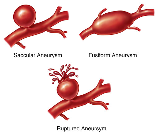
Accurate and efficient modelling of biomedical flows is of substantial interest because of its immediate applicability to a variety of fields, including the design of medical devices, the planning of surgical procedures and most fundamentally, the scientific understanding of healthy and diseased biological function. The complexity in this problem arises from the fact that physically-interesting flows occur in complex, patient-specific geometries and often occur in conjunction with other physics such as the finite deformation of the vascular walls and biochemical reaction-diffusion processes.
The primary aim of our research is the development of a robust computational framework for biomedical flow simulation and apply it to our current problem of interest: understanding how blood flow in an artery affects the formation and growth of aneurysms.

Such a problem motivates the need for accurate computation of quantities that are implicated in the growth of aneurysms (such as the shear forces exerted by the blood flow on their vessel walls and the stretch of the arterial walls due to normal pressure). We term these quantities of interest, “goal quantities.” Central to computing these quantities accurately are adaptive mesh techniques based on a posteriori error estimates, which rely on estimates of the errors in computed physical goal quantities to determine regions where the error needs to be reduced. These estimates are calculated from the computed solution and the solution of an auxiliary (dual) problem containing information about the stability of the flow equations being solved and the goal quantity expressed as a functional. Briefly, we use the fact that the error in the specified goal functional is the residual of the dual solution:
\begin{align} \mathcal{M}(u_{h}) - \mathcal{M}(u) & = \mathcal{M}(u_{h} - u)\\ & = a^{*}(z, u_{h} - u)\\ & = a(u_{h} - u, z)\\ & = a(u_{h}, z) - a(u, z)\\ & = a(u_{h}, z) - L(z)\\ & = r(z), \end{align}
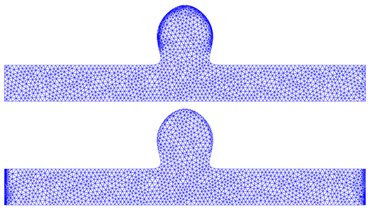
You can watch a talk I’ve given about this to better clarify concepts and see how we apply this general theory to equations modelling fluid flow. Applying our adaptive scheme to a 2D representation of an aneurysm results first in a simulation of the blood flow through the diseased vessel.
It also results in the construction of optimal computational meshes, which allow us to compute quantities related to aneurysm growth to a specified accuracy requirement with minimal computational work. Notice that the optimal mesh changes with the goal of our computation.

Algorithmic and software design lessons learnt from this project have been incorporated into CBC.Flow, a Python application written atop the FEniCS Project and distributed under the GNU GPL. It allows a user to easily pose and solve fluid flow problems with a syntax that is close to our automated hyperelasticity solver, CBC.Twist. The following is an example.
# Import utility classes from cbc.flow
from cbc.flow import *

# Define the flow problem
class Channel(NavierStokes):

    def mesh(self):
        return UnitSquare(16, 16)

    def viscosity(self):
        return 1.0 / 8.0

    def velocity_dirichlet_values(self):
        return [(0, 0)]

    def velocity_dirichlet_boundaries(self):
        return ["x[1] == 0.0 || x[1] == 1.0"]

    def pressure_dirichlet_values(self):
        return [1, 0]

    def pressure_dirichlet_boundaries(self):
        return ["x[0] == 0.0", "x[0] == 1.0"]

    def velocity_initial_condition(self):
        return (0, 0)

    def pressure_initial_condition(self):
        return "1 - x[0]"

    def end_time(self):
        return 0.5

    def __str__(self):
        return "Pressure-driven flow across a channel"

# Setup and solve problem
problem = Channel()
u, p = problem.solve()